Download Lake Erie Ice Cover Data

ice_cover-erie.R

library(rvest)
library(ggplot2)

url <- "https://coastwatch.glerl.noaa.gov/statistic/statistic.html"
html <- read_html(url)
data_links <- html_attr(html_nodes(html, "table:nth-child(3) td a"), "href")

table_header <- readLines(paste0(gsub(basename(url), "", url), 
                                 data_links)[1])[6]
table_header <- unlist(strsplit(strsplit(table_header, "   ")[[1]], "  "))
table_header <- unlist(strsplit(table_header, " "))
table_header <- table_header[nchar(table_header) > 0][1:9]
table_header <- make.names(trimws(table_header))

get_page <- function(url, x){ 
    res <- read.table(paste0(gsub(basename(url), "", url), 
                                        data_links)[x], skip = 8)
    names(res) <- table_header
    res
}

res <- lapply(seq_len(length(data_links)), function(x) get_page(url, x))
res <- do.call("rbind", res)
res$date <- as.POSIXct(strptime(paste0(res$Year, "-", res$Day), 
                                format = "%Y-%j"))

# cleaning ####
names(res)

# template <- data.frame(Year = NA, Day = NA)
template_year <- rep(seq(res$Year[1], res$Year[nrow(res)]), each = 365)
template_day  <- rep(1:365, times = length(unique(res$Year)))
template <- data.frame(Year = template_year, Day = template_day)

res <- dplyr::left_join(template, res)
res_na_rle <- rle(as.numeric(is.na(res$Erie)))
res <- res[(res_na_rle$lengths[1] + 1):
               (nrow(res) - res_na_rle$lengths[length(res_na_rle$lengths)]),]

# Analysis ####
library(wql)
library(forecast)
library(ggfortify)
library(ggplot2)
library(dplyr)

res_ts <- ts(res$Erie, 
             frequency = 365)
res_ts <- interpTs(res_ts)

y <- msts(as.numeric(res_ts), seasonal.periods = c(365))
fit <- tbats(y)
fc <- forecast(fit)

plot(fc)

ggseasonplot(lag(res_ts, -50), continuous = FALSE) + 
  geom_hline(yintercept = 80)

plot(fc$mean, ylim = c(0, 100))
lines(fc$upper[,2], col = "red")
lines(fc$upper[,1], col = "blue")
# abline(h = 80)
abline(v = 10 + (which(fc$upper[,2] > 80)[1] / 365) + (26 / 365), 
       col = "red", lwd = 2, lty = 2)
abline(v = 10 + (which(fc$upper[,1] > 80)[1] / 365) + (26 / 365), 
       col = "blue", lwd = 2, lty = 2)

as.Date("2018-01-01") + ((which(fc$upper[,1] > 80)[1] / 365) + (26 / 365)) * 365
as.Date("2018-01-01") + ((which(fc$upper[,2] > 80)[1] / 365) + (26 / 365)) * 365

res_pred <- data.frame(date = seq(as.Date("2018-01-05"), 
                                  as.Date("2018-01-05") + 729, by = 1), 
                       Erie_mean = fc$mean, 
                       Erie_80 = fc$upper[,1])
res_pred$Year <- format(res_pred$date, "%Y")
res_pred$year_wrap <- c(rep(2017, 168), res_pred$Year)[1:nrow(res_pred)]
res_pred$day_wrap <- as.numeric(format(as.Date(res_pred$date) + 168, "%j"))

res$year_wrap <- c(rep(2007, 168), res$Year)[1:nrow(res)]
res$day_wrap <- as.numeric(format(as.Date(res$date) + 168, "%j"))

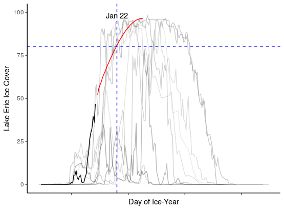
ggplot() + 
  geom_line(data = res[res$year_wrap != 2017,], 
            aes(x = day_wrap, y = Erie, 
                color = as.factor(year_wrap)), alpha = 0.4) + 
  geom_line(data = res[res$year_wrap == 2017,], 
            aes(x = day_wrap, y = Erie)) +
  geom_line(data = res_pred[res_pred$date < as.Date("2018-02-15"),], 
            aes(x = day_wrap, y = Erie_80), color = "red") +
  geom_hline(aes(yintercept = 80), 
             color = "blue", linetype = 2) + 
  geom_vline(aes(
    xintercept = res_pred[min(which(res_pred$Erie_80 > 80)), "day_wrap"]), 
             color = "blue", linetype = 2) +
  scale_color_grey(start = 0.8, end = 0.2) +
  ylim(0, 100) + ylab("Lake Erie Ice Cover") + xlab("Day of Ice-Year") +
  theme_classic() + theme(legend.position = "none", 
                          axis.text.x = element_blank()) +  
  geom_text(data = data.frame(x = 190, y = 98, lab = "Jan 22"), 
            aes(x, y, label = lab))

https://jsta.rbind.io/data/erie-ice_res.rds

https://robjhyndman.com/hyndsight/dailydata/