You signed in with another tab or window. Reload to refresh your session.You signed out in another tab or window. Reload to refresh your session.You switched accounts on another tab or window. Reload to refresh your session.Dismiss alert
A system usually has several different states it can inhabit. These states are called microstates. Microstates that are indistinguishable from each other are clubbed under a single macrostate, and the number of microstates that make up a macrostate is called the multiplicity of that macrostate.
For eg. if we have 100 coins, there is only one way in which every coin will be heads up. i.e. the macrostate of all coins being heads up has a multiplicity of 1. However, the macrostate of one coin being heads up and the rest tails up has a multiplicity of 100 because any one of the 100 coins could be heads up, and each of these represents a different microstate.
If we assume that every microstate is equally probable, a system is most likely to eventually end up in the macrostate with the highest multiplicity i.e. the most probable macrostate. The probability of this occurring is given by:
For the coin example, this works out to $\frac{\binom{N}{N/2}}{2^N}$, where $N$ is the number of coins. To evaluate this, we can use the Stirling approximation for $N!$, which is given by $\left(\frac{N}{e}\right)^N\sqrt{2\pi N}$.
Aside: To understand how the Stirling formula works, consider that $N!$ contains a product of $N$ numbers, which in the Stirling approximation is represented by $N^N$. Of course, this would mean we are overcounting quite a bit and so we "average" out the numbers by dividing each $N$ by $e$. Thus we get $\left(\frac{N}{e}\right)^N$. But this is too much of a correction and so we multiply the $\sqrt{2\pi N}$ term.
Cancelling out the terms, we get the final value as:
$$\sqrt{\frac{2}{\pi N}}$$
This is the probability of a system ending up in its most probable state. The probability decreases as $N$ increases. However, though the probability of ending up in the most probable state goes down, the probability of ending up in the neighbourhood of the most probable state rises.
We can illustrate this by considering a system of $N$ particles that can have $q$ energy states distributed among them. Assume that $q \gg N$. The total multiplicity of all states is
Now imagine that there were two systems, each with $N$ particles and $q_A$ and $q_B$ energy states each, and we'd like to see what the odds are of the systems settling into the most likely state of $q_A = q_B$.
This is a typical Gaussian distribution and drops off by $1/e$ at
$$N \left(\frac{2x}{q}\right)^2 = 1 \quad \text{or} \quad x = \frac{q}{2\sqrt{N}}$$
$\frac{q}{2\sqrt{N}}$ will be a very large number, but compared to the most probable state of $\frac{q}{2}$, it is $\frac{1}{\sqrt{N}}$ time smaller. For even a small macroscopic system, $N$ will be of the order of $10^{23}$ or more. Because the relative width of this Gaussian distribution scales as $1/\sqrt{N}$, the width of the peak is barely a hundred-billionth of the total possible range of states. This means that the system is overwhelmingly likely to end up in a state microscopically close and macroscopically indistinguishable from the most probable state due to sheer probability, making macroscopic fluctuations away from equilibrium effectively impossible.
Even if a system starts off in its most improbable state, it will invariably move towards the more probable states because there are exponentially more transitions leading to more probable states than there are transitions leading to less probable states. Eventually, the system must end up in its most probable neighbourhood.
This is the statistical interpretation of the second law of thermodynamics. While classical thermodynamics states that the entropy of an isolated system (like the universe) can never decrease, statistical mechanics frames this as the system overwhelmingly tending to evolve toward its most probable macrostate. Macroscopic decreases in entropy are theoretically possible but statistically so improbable that they are never observed.
Intensive & Extensive Properties
In thermodynamics, properties are classified based on how they change with the size or amount of matter in a system. Intensive properties do not depend on the amount of substance (e.g., temperature, pressure, density), while extensive properties scale with the size of the system (e.g., mass, volume, total energy). Their values add up when subsystems combine.
$T$, $P$, $\rho$ are intensive. $m$, $V$, $U$, enthalpy $H$, entropy $S$, and both Helmholtz and Gibbs free energies, $F$ and $G$, are extensive.
Key Rules: You can add or subtract between properties of the same class (provided their physical units match), but you cannot mix intensive and extensive properties in addition/subtraction.
Multiplying an intensive and extensive property gives another extensive property.
Dividing two extensive properties yields an intensive property.
State & Non-state Variables
State variables are independent of the process or path taken in state space to traverse between two states. They depend only on the initial and final states. $U$, $H$, $S$, $F$, $G$, $T$, $P$, $V$ are state variables. The cyclic integral of the differential of a state variable over a closed path in state space is always zero (e.g., $\oint dU = 0$).
Non-state variables depend on how the final state was arrived at. $Q$ and $W$ are non-state variables, which is why we represent them with inexact differentials ($\delta Q$, $\delta W$), representing an infinitesimal amount of energy transferred along a specific path in state space. If you went from state $A$ to $B$ via a reversible process compared to a non-reversible process, both the total $\int \delta Q$ and $\int \delta W$ would be different.
Temperature & Entropy
Entropy
The entropy of a system in equilibrium, where every accessible microstate is equally probable, is given by Boltzmann's entropy formula:
$$S = k_B \ln\Omega$$
For a system where microstates have varying probabilities, the general form (Gibbs entropy) is used:
$$S = -k_B \sum_s P_s \ln P_s$$
If we take the $k_B$ out of this formula and make it dimensionless, it is called the Shannon Entropy formula and is used in Information Theory. In this context, the logarithm is typically taken to base 2, and the resulting entropy is measured in "bits".
If $P_s$ is equal for all accessible microstates, then $P_s = \frac{1}{\Omega}$ for every state, and Boltzmann's and Gibb's formulations become identical. You can check this by substituting $P_s$ with $\Omega$ into the summation gives:
Since the sum is taken over all $\Omega$ states, the summation evaluates to $\Omega$ identical terms. This $\Omega$ cancels the $\frac{1}{\Omega}$ factor, yielding the original formula for equilibrium entropy.
In Short: When working with a system that has not yet reached equilibrium, we need to determine which states are more likely. We therefore calculate the entropy of various states using the multiplicities of those states to determine the final likely state i.e. the one with highest entropy. Once equilibrium is reached, the entropy of the system is given by the total multiplicity of all possible states, not just the most probable states. However, even if we do make our entropy calculations with the multiplicity of the most probable state, it is unlikely to be off by much because the total multiplicity is approximately the multiplicity of the most probable state.
Aside: In Information Theory, entropy is related to the "usefulness" or "surprise" of information. To understand this, consider asking for someone's birthday, and receiving one of the following answers:
"Sometime this year" (probability $P=1$)
"It is in January" (probability $P \approx 1/12$)
"It is on the 11th of a month" (probability $P \approx 12/365$)
The first statement is essentially useless and carries zero surprise, but has a probability of 1. The third statement is highly specific, has a much lower probability of being guessed randomly, and thus provides a high amount of information when revealed. The information content (or surprisal) of a specific outcome is proportional to $-\log_2 P$. The more improbable a piece of information, the more it helps constrain the uncertainty in information.
However, a highly improbable outcome, while carrying immense information value, occurs rarely. In information theory, we therefore define entropy as the uncertainty of the system. The more information we get from an improbable piece of content, the more we constrain the uncertainty. However, this improbable event is highly unlikely to take place. So we calculate the expected value of the information: $S = -\sum_s P_s \ln P_s$
Temperature
Previously, we considered two systems, each with $N$ particles and $q_A$ and $q_B$ energy states each. We saw that the two systems are highly likely to reach an equilibrium where they share the energy almost equally. If the energy was in the form of heat, we could just as well have said the two systems are extremely likely to end up at the same temperature. Temperature therefore is not defined as a fundamental quantity but as the heat (along a reversible path between states $A$ and $B$) required for a unit change in entropy:
$$T = \frac{\delta Q_{\text{rev}}}{dS}$$
and therefore:
$$dS = \frac{\delta Q_{\text{rev}}}{T}$$
This is the second law of thermodynamics.
When a process does not cause a change in volume or the number of particles in the system, the change in the system's energy $dU= \delta Q_{\text{rev}}$ and so $\frac{1}{T} = \frac{\partial S}{\partial U}$.
If more heat is required to change entropy, the system is at a higher temperature.
The other way to look at this is: a high temperature system will not lose much entropy for a large loss of heat. A low temperature system will gain a lot of entropy for the same gain in heat. Therefore, since the second law dictates that the entropy in the universe tends to increase, heat is likely to flow from high temperature to low temperature because that leads to a rise in entropy on the whole. Heat flow (except for microscopic random fluctuations) will end when the entropy lost/gained for a loss/gain of heat becomes equal for two systems, which means the total entropy no longer increases when heat flows. This means the two systems are at equal temperatures.
This is rather obvious in the intuitive case of heat transfer. But something similar can be seen in the case of a paramagnet, which gives a very non-intuitive picture of entropy.
Aside: Clausius' inequality evaluates the heat transfer relative to the temperature of the boundary where the heat exchange occurs during a cyclic process:
$$\oint \frac{\delta Q}{T} \le 0$$
For a process between two distinct states, this manifests as $dS \ge \frac{\delta Q}{T}$. (More on this later).
Paramagnets, Entropy & Temperature
Consider a paramagnetic substance under the influence of an external magnetic field. The individual atoms in the substance act like dipoles: they either align up i.e. in the direction of the magnetic field, or down i.e. in the opposite direction. Let us say the system starts off in the state where all dipoles are aligned with the magnetic field. This is a state with multiplicity $1$ and therefore, entropy of $0$. But its potential energy $U$ is at the minimum. This state is called lower lockout.
If we were to add energy to the system, the dipoles would begin to flip their orientation into the higher potential energy state where they oppose the magnetic field orientation. The multiplicity of the states that the system begins to occupy also increases as more atoms begin to flip. So the system is absorbing energy and its entropy is increasing, which means it starts to have a positive temperature.
Eventually, half the atoms will be flipped and half will be aligned with the magnetic field. This is a state of maximum multiplicity and entropy. The entropy cannot increase beyond this even with the addition of energy and this state is called saturation. Since the statistical definition of temperature is $\frac{1}{T} = \frac{\partial S}{\partial U}$, $T$ goes to infinity as the slope $\frac{\partial S}{\partial U}$ goes to $0$. Now let's say we continue to add more energy to the system. More atoms will continue to flip, but now the entropy begins to decrease. This means the slope $\frac{\partial S}{\partial U}$ becomes negative, so $T$ jumps to negative infinity. As energy continues to be added, entropy drops faster and faster, which means $T$ remains negative but approaches $0$ from below, and eventually reaches $0$ again in the case where every atom is flipped, a state with multiplicity $1$. This state is called upper lockout.
In fact, if we were to take a system at a very low positive temperature (where almost all atoms are aligned with the magnetic field) and suddenly reverse the magnetic field's orientation, the atoms are instantly left anti-aligned with the new field. This places the system immediately into a high-energy, low-entropy state, which is a negative temperature. The atoms would then begin to relax and flip to align with the new field direction, releasing a tremendous amount of energy as their entropy rises and the temperature approaches negative infinity, flips to positive infinity, and cools back down.
The temperature referenced in the spin system is the thermodynamic temperature, which is related to energy and entropy. This need not be the same as what we traditionally call "hot" and "cold", which is a specific manifestation of thermodynamic temperature known as kinetic temperature—it arises from the kinetic and translational movement of atoms and molecules.
If we graphed the spin system with entropy on the y-axis and the number of particles in a certain spin state (which is proportional to internal energy $U$) on the x-axis, the plot would be a parabolic arch.
The left end near the origin would have a positive $\frac{\partial S}{\partial U}$, so this state would be ready to absorb massive amounts of energy. The right side would have a negative $\frac{\partial S}{\partial U}$ and would be ready to release massive amounts of energy, though it is at a "negative temperature" or rather because it is at a negative temperature. The top of the graph would be flat and represent the maximum entropy and therefore infinite temperatures.
Note that this behaviour of negative temperatures is possible only because our system has an upper bound on energy and entropy. In general, in classical mechanics, the energy and entropy curves extend infinitely to the right and never reach a maximum peak or turn downward.
In solid-state physics, a material effectively contains two independent thermodynamic systems occupying the exact same physical space:
The Lattice: The physical structure of vibrating atoms. This unbounded system has a standard kinetic temperature.
The Spin System: The localized magnetic moments. This bounded system has its own independent thermodynamic temperature based strictly on the spin multiplicity.
Because the coupling (energy exchange) between the electron or nuclear spins and the physical lattice is often extremely weak, these two systems can be out of equilibrium. You can physically hold a crystal where the lattice is at a standard kinetic temperature of $300\text{ K}$, but by using radio-frequency pulses, you can drive the localized spin system into a population inversion, giving the spin system a negative thermodynamic temperature.
If the bounded spin system were to suddenly couple strongly to the unbounded physical lattice, energy would flow explosively from the negative-temperature spins into the positive-temperature lattice, rapidly heating the physical material until the spin "temperature" and lattice temperature equalized.
The First & Second Laws & the Thermodynamic Identity
The first law of thermodynamics states that energy is conserved. In thermodynamics, this means the change in the internal energy of the system is equal to the heat input to the system plus the work done on the system.
This always holds true for any closed system (except if you are looking at the expansion of the universe!).
The second law provides the macroscopic definition of entropy: $dS = \frac{\delta Q_{\text{rev}}}{T}$ or $\delta Q_{\text{rev}} = TdS$.
Mechanical work done on a fluid or gas system during a reversible volume change is:
$$\delta W_{\text{rev}} = -PdV$$
If we assume a closed system where the number of particles remains constant, we can substitute these into the first law to get:
$$dU = TdS - PdV$$
This is the fundamental thermodynamic identity. This is an equation written entirely in state variables. Therefore, though we derived it for a reversible process, this equation holds for the differential between any two neighbouring equilibrium states, regardless of whether the actual physical process connecting them was reversible or irreversible.
If we are considering an open system where the number of particles can change, the fundamental thermodynamic identity becomes:
$$dU = TdS - PdV + \mu dN$$
where $\mu$ is the chemical potential and $N$ is the number of particles in the system.
If the system involves some work other than the mechanical work to change volume, such as electrical work, these should also be included in the first law and the thermodynamic identity. They become:
Since the thermodynamic identity is generally written as an intensive property multiplied by the differential of an extensive property, this becomes: $dU = TdS - PdV + \mu dN + \phi dq$
Note: The thermodynamic identity is a relationship between state variables, meaning it is mathematically valid for evaluating the difference between the endpoints of any process, whether reversible or irreversible, provided the initial and final states are in thermodynamic equilibrium. By equilibrium, we mean uniform intensive variables, i.e. $T$, $P$ and $\mu$ are uniform throughout the system. If the system is not in equilibrium, for example if there are massive temperature gradients, pressure waves, and turbulent vortices throughout the volume, then the system as a whole does not possess a single, globally defined temperature or pressure that can be utilized in the equation. In such cases, we may be able to assume "local thermodynamic equilibrium," where the system is mathematically divided into infinitesimally small volume elements that are treated as being locally in equilibrium, allowing the identity to be applied differentially across spatial gradients.
Note on Pressure: You can isolate the formula for pressure from the fundamental thermodynamic identity ($dU = TdS - PdV + \mu dN$). By holding entropy and particle number constant ($dS = 0$, $dN = 0$), you get:
Pressure is therefore the energy needed to make a unit change in volume.
Note on Chemical Potentials: The chemical potential of a particle can be deduced by analyzing chemical reactions involving that particle in equilibrium. For example, when an electron transitions to a lower energy state, a photon is emitted:
$$e^- \rightleftharpoons e^- + \gamma$$
At thermal and chemical equilibrium, the sum of the chemical potentials of the reactants must equal the products:
$$\mu_e = \mu_e + \mu_\gamma$$
Which dictates that $\mu_\gamma = 0$. Photons in a thermal cavity have a chemical potential of zero because their particle number is not conserved; they can be freely created or destroyed to minimize the free energy of the system.
Similarly, assuming the chemical potential of a neutrino ($\nu$) and its antineutrino ($\bar{\nu}$) are equal ($\mu_\nu = \mu_{\bar{\nu}}$), we can look at their annihilation reaction:
$$\nu + \bar{\nu} \rightleftharpoons \gamma$$
This implies:
$$2\mu_\nu = \mu_\gamma = 0$$
Which means the chemical potential $\mu_\nu = 0$ for both neutrinos and antineutrinos in thermal equilibrium.
Thus, temperature is the driving potential for heat, pressure for volume and chemical potential for diffusion.
For a system in equilibrium, the internal energy $U$ can be expressed by the Euler relation:
$$U = TS - PV + \mu N$$
The Euler relation is not independent of the thermodynamic identity. It is a direct mathematical consequence of the fact that $U$, $S$, $V$, and $N$ are extensive properties.
If you scale the size of a system by a factor of $\lambda$, all extensive properties scale by that exact same factor. Therefore:
In multivariable calculus, a function that behaves this way is called a homogeneous function of degree one. According to Euler's theorem for homogeneous functions, if you differentiate this scaling equation with respect to $\lambda$ and then set $\lambda = 1$, the math strictly dictates that:
$$U = TS - PV + \mu N$$
Taking the total differential of this equation yields $dU = TdS + SdT - PdV - VdP + \mu dN + Nd\mu$. Subtracting the thermodynamic identity from this gives the Gibbs-Duhem relation:
$$SdT - VdP + Nd\mu = 0$$
This equation serves as a constraint on the intensive properties, i.e. $T$, $P$ and $\mu$ cannot vary independently of each other. If you change any two, the change in the third is already determined.
Now, taking the thermodynamic identity and assuming that the number of particles does not change ($dN = 0$), we get:
$$dU = TdS - PdV$$
If the system is quasistatic, meaning any change made to the system is so slow that the system always has time to reach equilibrium after each infinitesimal step, the change will be reversible and we get: $\delta Q_{\text{in}} = TdS$ and $\delta W_{\text{on}} = -PdV$. Note that these hold true even when there is friction, provided we ignore the work done to overcome friction and the heat lost due to friction to "non-system" components (such as the piston head).
However, consider a non-quasistatic system, for example, one in which a piston is being rapidly compressed on a chamber of gas. The gas particles near the piston will be pushed to a higher pressure than the rest of the gas (since they do not have time to equilibrate), exerting an extra reverse pressure on the piston greater than the average equilibrium pressure of the chamber. Therefore, more force will be required to compress the piston compared to the quasistatic case. Since compression means $dV$ is negative, $-PdV$ is a positive value representing the reversible work. The actual work required for the compression will be greater that the quasistatic case, so $\delta W_{\text{on}} > -PdV$.
By the Clausius inequality ($dS \ge \frac{\delta Q}{T}$), the heat input will be $\delta Q_{\text{in}} < TdS$.
Therefore, even in a non-quasistatic case, the First Law $dU = \delta Q_{\text{in}} + \delta W_{\text{on}}$ still holds true, but the individual components map to the thermodynamic identity as inequalities: $\delta Q_{\text{in}} < TdS$ and $\delta W_{\text{on}} > -PdV$. The decreased heat input (or increased heat rejected) is perfectly counterbalanced by the increased work done on the system. Therefore, the thermodynamic identity still holds:
$$dU = TdS - PdV$$
Note that during this rapid compression, the system may not be in equilibrium. The thermodynamic identity can be applied only in systems in equilibrium. However, we can always rapidly compress the gas, and then wait for the system to equilibrate before applying the thermodynamic identity. This is fine since what we are interested in is really the relationship between the initial and final states.
Going back to our formula for entropy, $dS = \frac{\delta Q_{\text{rev}}}{T}$, we can see that $\delta Q_{\text{in}} < \delta Q_{\text{rev}}$ in the non-quasistatic case. Essentially, if a process is not reversible, we extract less heat from it (or must expel more heat) compared to the reversible case. But the rise in the system's entropy is still dictated by $\delta Q_{\text{rev}}$ , so we end up "paying" a penalty of entropy equivalent to the reversible case, even though we extract less useful heat from the process.
Enthalpy & Free Energies
Suppose we wanted to calculate the heat released when aviation fuel is burnt in a constant pressure situation. You could build a calorimeter, burn the exact fuel blend, and measure the temperature change. But if the fuel mixture changes slightly tomorrow, you must run the physical experiment again.
Ideally, we would like to have reference tables that tell us how much heat the chemical reaction will release. If we could reduce this to a formula based purely on state variables, we would have a deterministic framework. We could write equations to mix and match various chemicals and figure out how much heat each mixture will release without needing an experiment for every permutation.
From the first law and the thermodynamic identity, $dU = \delta Q + \delta W_{\text{total}}$. If the only work done is reversible expansion work, then $\delta W_{\text{total}} = -PdV$, and the heat input (or in the case of the aviation fuel example, the heat output) is $\delta Q = TdS$.
The trouble with using $U$ as a state variable is that the heat input to the system provides for the rise in internal energy as well as for the expansion work done to accommodate the system's changing volume. Therefore, $U$ does not equate to heat input.
Instead, if we had a variable $H$ (enthalpy) that also included the expansion work, such that:
$$dH = dU + PdV$$
then $dH = TdS$ which is just the heat input (output).
We therefore define $H$ as $U + PV$. Since $H$ is a state variable, we can look them up via tables and perform the mix and match calculations we want to so that fuels can mixed etc.
Note that taking the differential of this equation results in: $dH = dU + VdP + PdV$. However, enthalpy is usually utilized in isobaric systems where $dP = 0$, and this equation reduces to $dH = dU + PdV$ and therefore to $dH = \delta Q$ .
Similarly, we can define the Helmholtz Free Energy $F$ as the total reversible work done on the system when the temperature is constant (thus, the work includes the non-extractable work that was expended by the system in expanding the volume). If we had $dF = dU - TdS$, then since $dU = TdS - PdV + \delta W_{on}$, we are left with $dF = - PdV + \delta W_{on}$ which is the work done on the system (by let's say some electrical system for example) minus the work done by the system in expanding the atmosphere, or whatever other ambient setup, during the process.
We therefore define $F$ as $U - TS$. Note that taking the differential of this equation results in: $dF = dU -TdS -SdT$. However, Helmholtz Free Energy is usually utilized in constant temperature systems and this equation reduces to the previous one.
Next, we define the Gibbs Free Energy $G$ as the total useful work done on the system, (i.e. the work needed to expand the surrounding medium is not included), when temperature and pressure are constant. If we had $dG = dH - TdS$, then since $dH = TdS -PdV + \delta W_{other} + PdV$, we are left with $dG = W_{other}$ which is exactly the useful work done on the system (by let's say some electrical system for example).
We therefore define $G$ as $H - TS$. Note that taking the differential of this equation results in: $dG = dU + PdV + VdP -TdS -SdT$. However, Gibbs Free Energy is usually utilized in constant temperature and pressure systems and this equation reduces to the previous one.
Legendre Transforms Perspective: Another way of looking at these state variables is through Legendre transformations. The internal energy $U(S, V, N)$ depends on extensive variables.
Enthalpy ($H$) is useful for constant-pressure systems, swapping the extensive $V$ for its intensive conjugate $P$.
Helmholtz Free Energy ($F$) is useful for constant-temperature systems, swapping the extensive $S$ for its intensive conjugate $T$.
Gibbs Free Energy ($G$) is useful for systems at constant temperature and pressure (like most chemical reactions), swapping both $S$ and $V$ for their intensive conjugates $T$ and $P$.
Why the Legendre Transforms are useful? The Second Law of Thermodynamics dictates that an isolated system will spontaneously evolve to maximize its entropy. Consequently, for a system held at constant $S$ and $V$, equilibrium is reached when the internal energy $U$ is minimized.
However, if a system is not isolated (e.g., it is held at constant $T$ and $P$ in an open beaker), maximizing the entropy of the system is no longer the correct criterion for equilibrium, because the system is exchanging heat with the environment. You must account for the entropy of the universe.
The Legendre-transformed potentials natively account for this environmental exchange.
If a system is held at constant $T$ and $V$, it will evolve until the Helmholtz Free Energy ($F$) is minimized.
If a system is held at constant $T$ and $P$, it will evolve until the Gibbs Free Energy ($G$) is minimized.
The transformation mathematically guarantees that minimizing the new potential is strictly equivalent to maximizing the total entropy of the system plus the reservoir.
Besides this, in engineering and experimental physics, it is practically impossible to constrain or directly measure entropy. However, intensive variables like temperature and pressure can be directly controlled in an experiment or system.
Boltzmann Statistics
Let us say we want to calculate the probability of finding a system (for instance, an atom) in any particular microstate, when that system is in thermal equilibrium with a reservoir at a specified temperature. The atom could conceivably be found in any of its microstates, but some will be more likely than others, depending on their energies. For an isolated system, all accessible microstates are equally probable. Our atom is not an isolated system, but the atom and the reservoir together do make an isolated system.
From the entropy formula $S = k_B \ln\Omega$, we can write the multiplicity $\Omega$ of a state as:
$$\Omega = e^{S/k_B}$$
If we consider two possible microstates for our small system, state 1 with energy $E_1$ and state 2 with energy $E_2$, the probability of finding the system in either state is directly proportional to the number of accessible microstates (multiplicity) of the reservoir when the system is in that state. We can write the ratio of the reservoir's multiplicities as:
Because the system and the reservoir exchange energy, the First Law dictates that any energy gained by the system is lost by the reservoir: $\Delta U_R = -(E_2 - E_1) = -\Delta E_{\text{sys}}$. Assuming the reservoir is at a constant volume (no expansion work) and no new particles are being added to the system, the thermodynamic identity for the reservoir is $dS_R = \frac{dU_R}{T}$. Therefore, the change in the reservoir's entropy is $\Delta S_R = -\frac{\Delta E_{\text{sys}}}{T}$.
Substituting this into our ratio gives the relative probability of the system occupying state 2 compared to state 1:
If we assume a ground state of zero energy ($E_1 = 0$), we can write the unnormalized probability (the statistical weight) of the system occupying any higher energy microstate $n$ with energy $E_n$ as:
$$\text{Boltzmann factor} = e^{-E_n/k_BT}$$
To convert these relative weights into true probabilities, they must be normalized so that the sum of all probabilities equals $1$. We do this by defining a normalizing denominator $Z$, such that:
$$\sum_n \frac{e^{-E_n/k_BT}}{Z} = 1$$
Solving for $Z$ yields the sum of all Boltzmann factors for all possible microstates:
$$Z = \sum_n e^{-E_n/k_BT}$$
This sum $Z$ is called the Partition Function. $Z$ represents the effective number or probabilistically weighted sum of thermally accessible microstates available to a system, where higher-energy states are occupied exponentially less often.
The true probability $P_n$ of the system occupying microstate $n$ becomes:
$$P_n = \frac{1}{Z} e^{-E_n/k_BT}$$
This resulting probability distribution is called a Boltzmann distribution.
Aside: Partition functions for composite functions of say N distinguishable particles are given by $Z = Z_1Z_2Z_3...$ . When the particles are indistinguishable, the number of states reduces by $N!$, which we divide the previous equation by.
To find the average energy (i.e. the expectation value) of the whole system, we take the average weighted with probability as below (where $\beta$ stands for $\frac{1}{k_B T}$):
We can use the Boltzmann distribution to calculate the energy of our previous paramagnet example. Because the spin can only align parallel (spin-up) or anti-parallel (spin-down) to the magnetic field $B$, the magnetic moment component along the field $\mu_z$ is restricted to exactly $+\mu$ or $-\mu$.
This yields exactly two discrete energy states for a single particle:
Ground State (Spin-up): Aligned with the field. $E_{\uparrow} = -\mu B$
Excited State (Spin-down): Anti-aligned with the field. $E_{\downarrow} = +\mu B$
Since the energy of a dipole in a magnetic field is $E = -\mu_z B$, the average expected energy per particle is:
$$\langle E \rangle = -B \langle \mu_z \rangle = -\mu B \tanh\left(\frac{\mu B}{k_B T}\right)$$
For a macroscopic system of $N$ non-interacting spins, the total net magnetization $M$ is simply $N$ times the average individual moment.
At the lockout or low temperature limit and Magnetic Saturation ($T \to 0$), the argument of the function $\frac{\mu B}{k_B T}$ approaches infinity. Because $\lim_{x \to \infty} \tanh(x) = 1$, the magnetization evaluates to $M = N \mu$. All spins are perfectly aligned in the ground state. At thermal saturation and infinite temperature ($T \to \infty$), the argument $\frac{\mu B}{k_B T}$ approaches zero. Because $\tanh(0) = 0$, the net magnetization evaluates to $M = 0$. The exact cancellation of equal numbers of spin-up and spin-down particles yields zero net spin, maximizing entropy.
Aside: Note that $cosh$ and $tanh$ are also found in Special Relativity and its hyperbolic rotations. These two mathematical frameworks are united through Quantum Field Theory and Statistical Field Theory using a transformation known as a Wick rotation, where the relativistic/quantum time variable $t$ is matched with an imaginary thermal time ($t \to -i \hbar \beta$, where $\beta = \frac{1}{k_B T}$).
Rotational Energy of a Diatom
For a diatomic molecule like CO or HCl, the allowed rotational energies are $E(j) = j(j + 1)\epsilon$, where $j = 0, 1, 2, \dots$, and $\epsilon$ is a constant that is inversely proportional to the molecule's moment of inertia. The number of degenerate states for level $j$ is $(2j + 1)$.
For high temperatures, the energy spacing is very small compared to $k_B T$, so this sum can be approximated as an integral over a continuous variable $j$:
We make the substitution $x = \beta \epsilon j(j+1)$. Taking the differential gives $dx = \beta \epsilon (2j+1) dj$. This conveniently absorbs the degeneracy factor, transforming the integral to:
The result $\langle E_{\text{rot}} \rangle = k_B T$ agrees precisely with the equipartition theorem, since a diatomic molecule has two degrees of rotational freedom, each contributing $\frac{1}{2} k_B T$ to the average energy.
Equipartition Theorem
We can also apply this to derive the equipartition theorem. This theorem applies only to systems whose energy is in the form of quadratic "degrees of freedom," expressed as $E(q) = c q^2$, where $c$ is a constant coefficient and $q$ is any coordinate or momentum variable, like $x$, $p_x$, or $L_x$.
The partition function for this system is:
$$Z = \sum_q e^{-\beta E(q)} = \sum_q e^{-\beta c q^2}$$
To evaluate the discrete sum, we can multiply by $\Delta q$ inside the sum and divide by $\Delta q$ outside the sum. This prepares it to be approximated as a Riemann sum:
$$Z = \frac{1}{\Delta q} \sum_q e^{-\beta c q^2} \Delta q$$
Assuming $\Delta q$ is very small, we can convert this summation into an integral over all possible continuous values of $q$:
$$Z = \frac{1}{\Delta q} \int_{-\infty}^{\infty} e^{-\beta c q^2} dq$$
To evaluate this, we use $u$-substitution. Let $x = q\sqrt{\beta c}$. The differential is therefore $dx = dq\sqrt{\beta c}$, meaning $dq = \frac{dx}{\sqrt{\beta c}}$. Substituting these into the integral gives:
The function $e^{-x^2}$ is a Gaussian, and its integral over the entire real line evaluates exactly to $\sqrt{\pi}$. Therefore, the partition function evaluates to:
$$Z = \frac{1}{\Delta q} \sqrt{\frac{\pi}{\beta c}} = C \beta^{-1/2}$$
where $C$ is introduced as a constant abbreviation for $\frac{1}{\Delta q}\sqrt{\frac{\pi}{c}}$.
We can then calculate the average energy of this degree of freedom using the standard expectation value relation $\langle E \rangle = -\frac{\partial \ln Z}{\partial \beta}$:
$$\langle E \rangle = -\frac{1}{Z} \frac{\partial Z}{\partial \beta} = -\frac{1}{C \beta^{-1/2}} \frac{\partial}{\partial \beta} \left( C \beta^{-1/2} \right)$$
$$\langle E \rangle = -\frac{1}{C \beta^{-1/2}} \left(-\frac{1}{2}\right) C \beta^{-3/2} = \frac{1}{2} \beta^{-1} = \frac{1}{2} k_B T$$
The system-specific constants $c$, $\Delta q$, and $\sqrt{\pi}$ have all cleanly canceled out, proving that any quadratic degree of freedom contributes exactly $\frac{1}{2} k_B T$ to the average thermal energy of the system, independent of the mass or specific mechanics of the particle.
In general, the equipartition theorem applies only when the spacing between energy levels is much less than $kT$. In situations where the number of distinct states that have significant probabilities is too small, then the smooth Gaussian curve will not be a good approximation to the bar graph.
Partition Function & Free Energy
The partition function is closely related to the multiplicity of a system. While multiplicity represents the total absolute number of accessible microstates, the partition function represents the number of effective microstates a system can explore at a fixed temperature.
Just as taking the logarithm of multiplicity gives us entropy ($S = k_B \ln \Omega$), taking the logarithm of the partition function connects us to another state variable. Because $Z$ is evaluated at a constant temperature, it naturally relates to the macroscopic state potential that minimizes at constant temperature: the Helmholtz Free Energy, $F$.
$Z$ increases as $T$ increases. However $F$ decreases as $T$ increases. Therefore the fundamental equation linking microscopic statistical mechanics to macroscopic thermodynamics is in fact:
$$F = -k_B T \ln Z$$
where $k_BT$ ensures that dimensions match on both sides. Equivalently, this can be written as:
$$Z = e^{-F/k_B T}$$
The usefulness of the formula $F = -k_B T \ln Z$ is that from $F$ we can compute the entropy, pressure, and chemical potential using partial-derivative formulas. Because the fundamental thermodynamic identity for the Helmholtz Free Energy is $dF = -SdT - PdV + \mu dN$, holding two of the three extensive variables constant allows us to isolate the intensive variables:
This allows us to compute all the macroscopic thermodynamic properties of a system once we know its microscopic partition function.
Ideal Gas
For an ideal gas of N molecules, we have
$$Z = \frac{1}{N!} Z_1^N$$
where the energy state of each molecule can be split into an internal energy component and a translational kinetic energy component as $Z_1 = Z_{\text{tr}} Z_{\text{int}}$, where:
We ignore the internal energy states for now and focus on the translational states. We calculate the energy by considering the de Broglie wavelengths of a molecule in a box of length L. The longest wavelength will be double the length of the box and subsequent wavelengths will be integer divisions of this: $\lambda_n = \frac{2L}{n}, \quad n = 1, 2, \dots$.
The momentum is given by $p = h/\lambda$ and $p_n = \frac{h}{\lambda_n} = \frac{hn}{2L}$
The states of energy are given by:
$$E_n = \frac{p_n^2}{2m} = \frac{h^2n^2}{8mL^2}$$
Putting this into our partition function and converting the sum into an integral (assuming $kT$ and $L$ are high enough), we get
where $\ell_Q \equiv \frac{h}{\sqrt{2\pi mkT}}$ is the quantum length. Aside from the factor of $\pi$, it is the de Broglie wavelength of a particle of mass m whose kinetic energy is $kT$.
Aside: Classically, if you had some object that occupied a length of $\ell_Q$ in a box of length $L$, you would say the effective number of places you could find this object in is in one of the $L/\ell_Q$ cells. Classically, the $p,x$ phase space is continuous. However, quantum mechanics dictates that phase space is fundamentally pixelated due to the Heisenberg uncertainty principle ($\Delta x \Delta p \ge \frac{\hbar}{2}$). The minimum possible phase space volume (or area, in one dimension) that a single, distinct quantum state can occupy is exactly Planck's constant, $h$.
To find the effective number of accessible states, you calculate the total available phase space area and divide it by $h$. The maximum spatial uncertainty of the particle is simply the length of the box, $L$. At a given temperature $T$, the thermal momentum spread of the particle is $p_{\text{th}} = \sqrt{2\pi m k_B T}$ or $\frac{h}{\ell_Q}$.
The total thermally accessible phase space area is the product of the spatial and momentum extents: $L \times p_{\text{th}} = L \times \frac{h}{\ell_Q}$.
To find the number of states $Z$, you divide this total available area by the fundamental area of a single quantum state ($h$): $Z = \frac{L \times \frac{h}{\ell_Q}}{h} = \frac{L}{\ell_Q}$.
where $v_Q = \ell_Q^3 = \left(\frac{h}{\sqrt{2\pi mkT}}\right)^3$, is the quantum volume. This intuitively suggests that the number of effective translational states is just the volume of the box divided by the quantum volume.
We can write the partition function for one molecule and $N$ molecules as:
In the previous Boltzmann distribution, if we consider that new particles are being added to the system or exchanged with a reservoir, the relative probability of two states becomes:
To normalize the probabilities, we carry out the same operation as before and define a normalizing denominator, known as the Grand Partition Function ($\mathcal{Z}$):
To see how the probability of states varies in systems that exchange particles, we specifically look at fermions and bosons under specific conditions.
Fermi-Dirac Distribution
Returning to the Boltzmann distribution and accounting for the exchange of particles with a reservoir, we now look at a quantum system where the particle density is high for example when the available volume per particle is equal to or less than the quantum volume (the thermal de Broglie wavelength cubed).
If the particles are fermions, they must obey the Pauli Exclusion Principle, which states that only one particle can occupy a specific quantum state at a time. Therefore, for a particular single-particle state where the energy is $\epsilon$, the number of occupying particles $n$ can only be $0$ or $1$.
The grand partition function for this single state is:
We calculate the average number of particles in this state, called the expected occupancy number $\langle n_{\text{FD}} \rangle$, by taking the probability of occupancy ($n=1$) and multiplying by $1$:
Note that this is occupancy of a particular state of a given energy $\epsilon$, and not for some system with fermions occupying multiple energy states.
Behavior of the Fermi-Dirac Distribution:
If $\epsilon \ll \mu$, the exponential approaches $0$, and $\langle n \rangle \to 1$ (the state is fully occupied).
If $\epsilon \gg \mu$, the exponential dominates, and $\langle n \rangle \to 0$ (the state is empty).
If $\epsilon = \mu$, the exponential is $e^0 = 1$, yielding an exact $50%$ expected occupancy. The width of the transition (fall-off) from $1$ to $0$ is proportional to a few multiples of $k_B T$. At low temperatures, this fall-off is a very sharp cliff where the occupancy drops suddenly from $1$ to $0$ exactly at $\epsilon = \mu$.
To understand why this cliff changes shape with temperature, we must examine the physical behavior at $T = 0$. Because fermions obey the Pauli exclusion principle, no two particles can occupy the exact same quantum state. At absolute zero, a system of fermions will settle into the lowest possible energy configuration by filling the available energy states one by one from the ground state upward.
The energy of the highest occupied state in this absolute zero configuration is called the Fermi energy ($E_F$). At $T = 0$, the chemical potential is equal to this Fermi energy ($\mu = E_F$) because every new particle needs to have an energy at least equal to $E_F$ in order to occupy the next highest energy state. Every state below $\mu$ is strictly filled, and every state above $\mu$ is strictly empty. This solid block of occupied states in energy space is referred to as the Fermi sea. Note that $\mu$ changes as new fermions are added, i.e. with $n$ because each new fermion needs to have sufficient energy to enter the next higher energy state, and chemical potential is literally defined as the energy needed to add an additional particle.
When $T > 0$, thermal energy is introduced into the system. The typical thermal energy available to any single particle is on the order of $k_B T$. This energy allows fermions to potentially jump into higher, unoccupied energy states. However, for fermions buried deep in the Fermi sea (where $\epsilon \ll \mu$), a thermal fluctuation of $k_B T$ is insufficient to reach the empty states above the surface. Because all adjacent states are already occupied, the Pauli exclusion principle forbids the transition.
Therefore, only the fermions very close to the surface of the Fermi sea, pecifically those within an energy range of roughly $k_B T$ below $\mu$, have the opportunity to absorb thermal energy and jump into the empty states located just above the surface. As $T$ increases, the magnitude of $k_B T$ grows, increasing the "depth" from which particles can jump. This thermal excitation of surface fermions is what smooths out the sharp cliff, creating a tapered, symmetric transition in the occupancy distribution around $\epsilon = \mu$.
Bose-Einstein Distribution
For bosons, there is no restriction on occupancy, so $n$ can range from $0$ to $\infty$ for a particular state of energy $\epsilon$. The grand partition function for a single state becomes an infinite geometric series:
Occupancy approaches infinity as $\epsilon$ approaches $\mu$ from above.
The chemical potential $\mu$ must always be less than or equal to the ground state energy (usually $\epsilon \ge 0$, so $\mu \le 0$). If $\epsilon$ were less than $\mu$, the resulting occupancy would be negative, which is physically impossible.
The Classical Limit: When the system is sparse or at high temperatures, the available states vastly outnumber the particles. In this regime, $(\epsilon - \mu) \gg k_B T$, making the exponential term $e^{(\epsilon - \mu)/k_B T}$ much larger than $1$. The $\pm 1$ in the denominators of both distributions becomes negligible, and both distributions collapse into the classical Boltzmann statistics $\langle n \rangle \approx e^{-(\epsilon - \mu)/k_B T}$
Photons & Blackbody Radiation
Photons are bosons whose chemical potential is zero ($\mu = 0$) because their number is not conserved. The energy of a photon is a multiple of $hf$. For a single electromagnetic mode (a specific frequency $f$), the partition function is the sum over all possible numbers of photons (essential infinite) in that mode:
The average number of photons per energy state (mode) is given by:
$$\langle N \rangle = \frac{1}{e^{\beta hf} - 1}$$
which is the standard formula from the Bose-Einstein distribution.
This is called the Planck Distribution, which shows that the short-wavelength (high-frequency) modes of the electromagnetic field, where $hf \gg k_B T$, are exponentially suppressed.
If we confine the system to a 3D box of side length $L$, we use the same quantized momentum approach as for an ideal gas. For photons, $E = pc$. Since $p = \frac{h}{2L}\sqrt{n_x^2 + n_y^2 + n_z^2} = \frac{hn}{2L}$, the allowed energies are:
$$E = \frac{hc n}{2L}$$
To get the total energy, we integrate over the continuous approximation of the modes in 3D space, accounting for the two polarization states of a photon. Integrating this gives the energy density with respect to volume as:
The integrand is the Planck spectrum, which gives the intensity of radiation as a function of photon energy. Integrating the spectrum between two energies (or frequencies) gives the total energy emitted in that interval.
Plotting the spectrum with intensity on the y-axis and energy along the x-axis shows a peak intensity at $E \approx 2.82 k_B T$, with a long tail tapering off to the right, called the Wien Tail. The general height of the plot and the total intensity increase with temperature. If plotted against wavelength, the peak shifts to the towards shorter wavelengths) as $k_B T$ increases. This is encoded in Wien's Displacement Law, $\lambda_{\text{max}} T = \text{constant}$. Thus, you can guess the temperature of a hot object by looking at the colour of its dominant emitted photons.
Evaluating the definite integral above gives us the exact formula for the total energy density:
Aside from the numerical constants, you can intuitively arrive at this functional form by looking at the average energy per photon, which is proportional to $k_B T$. The total number of photons can be estimated by dividing the total volume $V$ by the quantum volume. The quantum volume is the cube of the quantum length (the thermal de Broglie wavelength), given roughly by $\frac{hc}{E} \approx \frac{hc}{k_B T}$.
Using the formula for the energy density in a box, we can also obtain the power emitted by a blackbody per unit area, which has a similar dependence on $T^4$. First, we can see qualitatively that the photons emitted by a blackbody are the same as the photons emitted by a small hole in a cavity containing a photon gas.
Suppose a hole in a photon box and a blackbody are at the same temperature, facing each other. Each object emits photons, some of which are absorbed by the other. If the objects are the same size, each will absorb the same fraction of the other's radiation. If they did not emit the exact same amount of power, more energy would flow one way or the other and the temperatures would no longer be equal, violating the Second Law of Thermodynamics.
Thus, all we need to do is calculate the power emitted per unit area by the hole in the box of photons. With some geometry to account for the flux escaping through the hole, this leads directly to the Stefan-Boltzmann Law:
$$P = \sigma \epsilon A T^4$$
where $A$ is the area and $\epsilon$ is the emissivity. $\epsilon$ is $1$ for a perfect blackbody. For real materials, $\epsilon < 1$, as such materials both emit and absorb less radiation due to their propensity to reflect incoming photons. A perfectly reflective surface would have an emissivity of $0$.
Ising Model of Ferromagnetism
In our earlier paramagnet example, we assumed that each dipole orients itself independently of the orientation of its neighbours. In the real world, dipoles are influenced by their neighbours. In some materials, this is due to ordinary magnetic dipole-dipole forces. In more dramatic examples (such as iron), this is driven by the quantum-mechanical exchange interaction involving the Pauli exclusion principle. Either way, there is a contribution to the energy that depends on the relative alignment of neighbouring dipoles.
When neighbouring dipoles align parallel to each other, even in the absence of an external field, we call the material a ferromagnet. When neighbouring dipoles align antiparallel, we call the material an antiferromagnet.
When seen as a whole, a ferromagnetic material may not exhibit any net macroscopic magnetization. This is because the dipoles group into microscopic clusters called domains. While each domain is locally magnetized, adjacent domains orient in different directions to minimize the macroscopic magnetostatic energy (the stray magnetic field extending outside the physical material). Put together, their vector sum cancels out.
If you apply a sufficiently strong external magnetic field, the domain walls shift. Domains aligned with the field grow at the expense of others, and the material becomes permanently magnetized even after the external field is removed. However, at temperatures beyond a critical threshold called the Curie temperature ($T_C$), thermal fluctuations overwhelm the quantum exchange interactions. The domain structures break down, and the material undergoes a phase transition, acting strictly as a paramagnet.
The 1-D Ising Model
The Ising model is a mathematical approximation of a ferromagnet assuming that dipoles have a strictly defined preferred axis and can only align ($+1$) or anti-align ($-1$) with it. The energy due to the interaction of a pair of neighbouring dipoles is $-\epsilon$ when they are parallel and $+\epsilon$ when they are antiparallel.
If we label the spin state of two neighbouring dipoles as $s_1$ and $s_2$ (where $s_i \in {+1, -1}$), the interaction energy between them is:
$$E = -\epsilon s_1 s_2$$
Assuming all $N$ dipoles are arranged in a single 1-D line, the partition function $Z$ sums over all possible spin configurations:
where the total internal energy is $U = -\epsilon \sum_{i} s_i s_{i+1}$.
By factoring out the summations from the end of the chain, the summation for the final dipole's interaction with the penultimate dipole yields the two states $+1$ and $-1$:
$$e^{\beta \epsilon s_{N-1}} + e^{-\beta \epsilon s_{N-1}} = 2\cosh(\beta \epsilon)$$
Pulling out each sum iteratively, we find that the partition function for a large $N$ chain is exactly:
$$Z = 2^N (\cosh(\beta \epsilon))^{N-1} \approx (2\cosh(\beta \epsilon))^N$$
Using $\langle E \rangle = -\frac{\partial \ln Z}{\partial \beta}$, the average expected energy is:
$$\langle E \rangle = -N\epsilon \tanh(\beta \epsilon)$$
Both $Z$ and $\langle E \rangle$ for this system are mathematically identical to a two-state paramagnet, simply replacing the external magnetic interaction energy $\mu B$ with the neighbour-neighbour interaction energy $\epsilon$. However, a major theoretical result of this 1-D model is that it produces zero spontaneous magnetization for all $T > 0$. A 1-D chain cannot sustain long-range ferromagnetic order because a single flipped spin physically breaks the chain of communication, and the entropy gained by flipping outstrips the energy penalty.
Mean Field Approximation (Higher Dimensions)
To observe a true phase transition (a sudden onset of magnetization at the Curie temperature), we must model higher dimensions: a 2-D lattice (4 nearest neighbours), a 3-D simple cubic lattice (6 neighbours), 8 in a 3-D body-centered lattice and 12 in a 3-D face-centered lattice. Let $q$ represent the number of nearest neighbours (the coordination number).
A powerful simplification used here is the Mean Field Approximation. The trick is to assume that all surrounding dipoles act as a single, uniform effective field possessing an average spin $\bar{s}$.
The energy of a single dipole of interest interacting with its $q$ neighbours is:
The expected average spin of this specific dipole is calculated probabilistically:
$$\langle s \rangle = \frac{(+1)e^{\beta \epsilon q \bar{s}} + (-1)e^{-\beta \epsilon q \bar{s}}}{Z} = \tanh(\beta \epsilon q \bar{s})$$
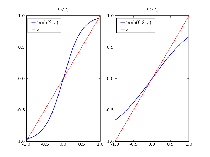
The core logic of the mean field approximation demands self-consistency: there is nothing special about this dipole. Its expected spin $\langle s \rangle$ must exactly equal the average surrounding spin $\bar{s}$. This gives us a transcendental equation:
$$\bar{s} = \tanh(\beta \epsilon q \bar{s})$$
Spontaneous Symmetry Breaking
Graphing both sides of this transcendental equation (plotting $y = \bar{s}$ and $y = \tanh(\beta \epsilon q \bar{s})$ against $\bar{s}$) reveals the system's phase behavior:
The slope of the hyperbolic tangent at the origin is $\beta \epsilon q$.
$\beta \epsilon q < 1$, the only intersection point is at the origin ($\bar{s} = 0$). The material is paramagnetic.
When $\beta \epsilon q > 1$, the slope at the origin is steeper than 1. The curves intersect at the origin and at two symmetrical non-zero points in the first and third quadrants. The solution at the origin becomes mathematically unstable; any infinitesimal thermal fluctuation will push the system into one of the two non-zero stable states ($+\bar{s}$ or $-\bar{s}$).
When a system inherently possesses symmetric equations but is forced to "choose" a distinct, non-symmetric state (like strictly spin-up or spin-down) at low temperatures, we say that the symmetry is spontaneously broken.
Solving for the boundary condition where the slope exactly equals 1 ($\beta \epsilon q = 1$) yields the critical Curie temperature:
$$T_C = \frac{q \epsilon}{k_B}$$
This confirms that the phase transition temperature is directly proportional to both the strength of the atomic interaction ($\epsilon$) and the geometric density of the lattice structure ($q$).
Critical Droplet Size
If a weak magnetic field is applied to a ferromagnet, and suppose all dipoles are currently anti-aligned with it, each individual dipole will have a very minimal tendency to flip and align with the magnetic field. Though the energy lost from aligning with the magnetic field should increase the probability of that state via the Boltzmann distribution, the energy gained from being anti-aligned with all its neighbours more than negates that gain. Thus, the local energy penalty creates the barrier. The higher the external magnetic field strength, the lower this barrier. For very weak external fields, the barrier is quite high and even if the dipole absorbs enough random thermal energy from its environment to flip, it will most likely flip back because the energy lost from re-aligning with its neighbours dictates that re-alignment would be the more probable state.
The single flipped dipole is an unstable "sub-critical" fluctuation. It appears and vanishes constantly, never triggering a cascade. The exact physical framework, known as nucleation theory, says that to trigger a cascade, the system must flip a cluster of dipoles, not just one. The stability of this cluster is governed by the mathematical competition between its surface area and its volume.
Imagine a small spherical cluster of flipped dipoles of radius $r$. The exchange penalty only occurs at the boundary of the cluster, where flipped dipoles touch unflipped ones. This energy cost grows with the surface area of the cluster: $\Delta E_{\text{cost}} \propto r^2$.
Every dipole inside the cluster gains energy from aligning with the weak external field. This energy gain grows with the total volume of the cluster: $\Delta E_{\text{gain}} \propto -r^3$.
Because $r^3$ grows faster than $r^2$, there is a mathematical tipping point where volume wins over area. If you plot the total energy of the cluster as it grows, the energy initially rises (cost dominates) to a maximum peak, and then plunges downward (gain dominates). That peak defines the critical radius ($r_c$).
For a cascade to occur, a statistically massive and exceptionally rare thermal fluctuation must flip a large enough cluster of dipoles simultaneously (or in rapid sequence) to exceed $r_c$. From this point onward, the cluster stabilizes. It aggressively recruits neighbouring dipoles, and the domain wall sweeps across the material, causing the macroscopic cascade. However, this thermal fluctuation is astronomically rare.