Last active
April 25, 2018 18:38
-
-
Save wbadry/9797a68fcbe945deafc680df5a7723c0 to your computer and use it in GitHub Desktop.
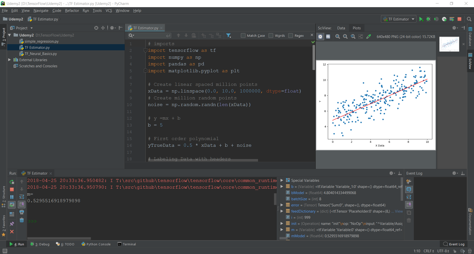
This is an example of using TensorFlow for simple Linear Regression of 1M points
This file contains hidden or bidirectional Unicode text that may be interpreted or compiled differently than what appears below. To review, open the file in an editor that reveals hidden Unicode characters.
Learn more about bidirectional Unicode characters
| # imports | |
| import tensorflow as tf | |
| import numpy as np | |
| import pandas as pd | |
| import matplotlib.pyplot as plt | |
| # Create linear spaced million points | |
| xData = np.linspace(0.0, 10.0, 1000000, dtype=float) | |
| # Create million random points | |
| noise = np.random.randn(len(xData)) | |
| # y =mx + b | |
| b = 5 | |
| # First order polynomial | |
| yTrueData = 0.5 * xData + b + noise | |
| # Labeling Data with headers | |
| x_df = pd.DataFrame(data=xData, columns=['X Data']) | |
| y_df = pd.DataFrame(data=yTrueData, columns=['Y']) | |
| # Joining input and output as columns | |
| myData = pd.concat([x_df, y_df], axis=1) | |
| # Get random initial values for b and m | |
| rValue = np.random.randn(2) | |
| m = tf.Variable(rValue[0]) | |
| b = tf.Variable(rValue[1]) | |
| # Number of points per batch | |
| batchSize = 8 | |
| xph = tf.placeholder(dtype=tf.float64, shape=[batchSize]) | |
| yph = tf.placeholder(dtype=tf.float64, shape=[batchSize]) | |
| # Create the first order model | |
| y_model = m * xph + b | |
| # Loss function | |
| error = tf.reduce_sum(tf.square(yph - y_model)) | |
| # Optimizer | |
| optimizer = tf.train.GradientDescentOptimizer(learning_rate=0.001) | |
| train = optimizer.minimize(error) | |
| # Create a session | |
| sess = tf.Session() | |
| # Initialize all variables | |
| init = tf.global_variables_initializer() | |
| sess.run(init) | |
| # Start optimization | |
| numberOfBatches = 1000 | |
| for i in range(numberOfBatches): | |
| randIndices = np.random.randint(0, len(xData), size=batchSize) | |
| feedDictionary = {xph: xData[randIndices], yph: yTrueData[randIndices]} | |
| sess.run(train, feed_dict=feedDictionary) | |
| # Get optimal m and b | |
| [mModel, bModel] = sess.run([m, b]) | |
| print('m=') | |
| print(mModel) | |
| print('\n') | |
| print('b=') | |
| print(bModel) | |
| # Plotting result | |
| yModel = mModel * xData + bModel | |
| # plotting sample of the generated data | |
| plt.figure() | |
| myData.sample(250).plot(kind='scatter', x='X Data', y='Y') | |
| # plt.plot(xData, yTrueData, '*') | |
| plt.plot(xData, yModel, 'r') | |
| plt.show() |
Author
Sign up for free
to join this conversation on GitHub.
Already have an account?
Sign in to comment
Code result using pyCharm